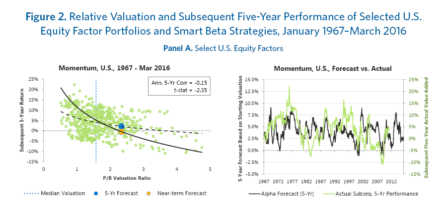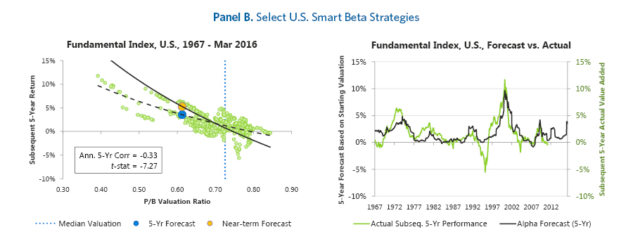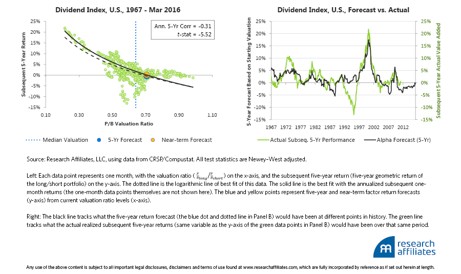
Over the past half-century, almost all of the eight factors and eight smart beta strategies we study exhibit a negative relationship between starting valuation and subsequent five-year performance.
Today, valuations of many of the most popular factors and smart beta strategies are well above their historical norms, forecasting lower future returns.
Our findings are robust for both factors and smart beta strategies across horizons out to five years, using both a simple price-to-book ratio and an aggregate valuation measure, in U.S., developed ex U.S., and emerging markets.
This is the second of a series on the future of smart beta.
In our first article in this series—“How Can ‘Smart Beta’ Go Horribly Wrong?” 1—we show, using U.S. data, that the relative valuation of a strategy (in comparison with its own historical norms) is correlated with the strategy’s subsequent return at a five-year horizon. The high past performance of many of the increasingly popular factor tilt and so-called smart beta2 strategies came, in large measure, from rising valuations. These excess returns are an “alpha mirage” attributable to the strategies’ becoming more expensive relative to the market. Even the statistical significance of past performance was an illusion driven by rising relative valuation levels! Today, only the value category shows some degree of relative cheapness, precisely because its recent performance has been weak.
Product proliferation in factor investing and “smart beta” create two interconnected risks. First, few if any products will be introduced without having wonderful historical returns. In many cases, these returns are a consequence of rising valuations. Basically, in product creation our industry is data mining on past performance. This selection bias creates an illusion of high past alpha that often disappears when we subtract the effect of rising relative valuations. The alpha mirage creates implausible expectations for investors, who are disappointed when realized returns almost inevitably fall short, and they switch strategies, typically at a substantial cost.
The second risk is far more dangerous: investing when relative valuations are at an extreme—aka performance chasing. Investing in overpriced strategies is value destroying. High past alpha can quickly become negative future alpha. Investors lock in their loss when they move on to the next strategy with wonderful past returns. Just like in selecting stocks, asset classes, managers, and funds, we are exposed to the same perils when we select factors and smart beta strategies. We marvel that these observations are controversial in some circles.
In this article, we present evidence that the relationship between current relative valuation and subsequent performance for both factors and smart beta strategies is robust over horizons shorter than five years and using valuation measures other than price-to-book (P/B) ratio. Furthermore, we unequivocally find statistically significant correlations in out-of-sample international and emerging markets similar to those we find in U.S. markets, although the timing signal has unsurprising uncertainty in any forecast of alpha (it’s pretty noisy). We add two new factors and two new smart beta strategies to our analysis.
The practical implication for investors is simple: valuations matter. They matter in all markets, both U.S. and non-U.S., developed and emerging, and they matter for strategies and factors, every bit as much as they matter when choosing managers, funds, and individual stocks. Valuations matter because they are predictive of future returns. Today, valuations of many of the most popular factors and smart beta strategies are well above historical norms. We have demonstrated that these high valuations are indicative of lower future returns, even if they are not able to provide any prescience on picking peaks or troughs. We do know, however, that valuations are considerably cheaper than historical norms—virtually universally—for the currently unpopular value factor and for the value-tilt smart beta strategies. No performance chasers found here!
The Value Factor: Forecast vs. Actual Alpha
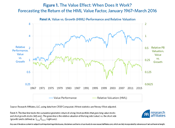
To provide context for a discussion and demonstration of the predictive ability of starting valuations to forecast five-year performance, we use the value factor to illustrate one of our major findings from the first article. The information in Figure 1, Panels A and B, will be familiar to those readers. The blue line in Panel A shows the return of the classic Fama–French HML (high minus low) value factor, which compares a capitalization-weighted portfolio of the 30% cheapest stocks (high book-to-price ratio) to a cap-weighted portfolio of the 30% most expensive stocks (low book-to-price ratio).

We can see in Panel A that the ups and downs of the performance of the value portfolio relative to the performance of the growth portfolio (the blue line) and the ups and downs of relative valuation of value relative to growth (the green line) fit like a glove. The rolling 12-month correlation between the two is a lofty 74%. Stop the presses! Whenever value is becoming more expensive relative to growth, it’s outperforming, with few exceptions. Reciprocally, whenever value is underperforming growth, it’s because it is becoming cheaper, with few exceptions.
The performance of the value portfolio relative to that of the growth portfolio starts at 1 in 1967 (left-hand log scale) and ends a bit over 3 in March 2016. The value portfolio over the 49¼ years from 1967 to March 2016 would have generated three times the income of the growth portfolio over the same period for an investor holding the long–short value factor portfolio.3 Surprisingly, this happened in the context of value finishing cheaper than it started a half-century ago. We call this the “wedge,” the manifest spreading of the difference between the blue relative-performance line and the green relative-valuation line. A large wedge is evidence of structural alpha, not to be confused with the situational alpha of a factor adding value only because it is becoming more expensive!
The green line in Panel A traces a new (as far as we know) phenomenon that has received little or no attention in the academic or practitioner literature: the trajectory of relative valuation, measured by P/B, of the value portfolio relative to the growth portfolio. The green line ranges as low as 0.08 and as high as 0.32 (right-hand log scale), meaning that the P/B ratio of the value portfolio has ranged between 8% and 32% of the P/B ratio of the growth portfolio. Put another way, using the reciprocal of these numbers, growth has commanded anywhere from a lofty 12 times to a mere 3 times the valuation multiple of value. It might seem that a 3-to-1 ratio between the valuation of growth relative to value is a big spread, but it’s not; the spread averages closer to 5 to 1.
Each dot in the scatterplot in Panel B represents a month from January 1967 to March 2011. The horizontal axis measures the relative valuation of value versus growth, ranging as just noted from 0.08 to 0.32. The vertical axis measures the subsequent five-year relative performance of value versus growth (hence the end date of 2011). Each data point represents a monthly observation of overlapping five-year periods, creating a visual illusion of more observations than we actually have. The dashed line shows the regression fit between the two; a lower starting valuation for value relative to growth strongly correlates with higher subsequent five-year performance.
The solid line in Panel B shows the regression of starting valuation with near-term relative performance of value relative to growth, based on annualizing the subsequent one-month relative performance; the individual plot points are not shown because monthly returns are very noisy. The linkage between starting valuation and subsequent near-term performance is also strong and fades surprisingly little as we move to a five-year forecasting span. Not wishing to delve too deeply into causality, this would nevertheless seem to be strong evidence for an inefficient market; that is, when value is cheap, its subsequent performance is strong, and when it’s fully priced (i.e., above roughly one-fourth the valuation of growth), the value effect disappears. As contrarians, we appreciate this inefficiency.
The blue and yellow dots on the regression lines correspond to the relative valuation of the value factor, equal to 0.13 in March 2016, comfortably in the bottom decile of historical relative valuation. Value’s corresponding future performance, assuming the historical relationships between starting relative valuation and subsequent relative performance hold, should outpace growth by nearly 8% a year looking ahead five years. Of course, these results include look-ahead bias, so we should haircut these expectations a bit. Also, past is not prologue: things are always a little “different this time.” Accordingly, we caution against over-reliance on the specific “forecast” of returns. Nonetheless, when the indication is this strong, we think the finding is highly likely to be at least directionally correct!
Now we move into new territory. Using the regressions in Panel B to convert starting valuation into a rolling five-year forecast of relative performance, we plot in Panel C the historical forecasts of relative performance, compared to the actual five-year outcome from 1967 through March 2016. The fit is pretty good, although the range of outcomes is much wider than the range of forecasts. Because this is an in-sample test, look-ahead bias is embedded in our regressions, overstating the fit between forecast and subsequent outcome.4
The Relationship of Valuation to Performance
Value investing involves selecting and purchasing cheap companies whose stock prices are low relative to their fundamentals; typically, this is defined as P/B, price-to-earnings (P/E), dividend yield, and/or other metrics. Ample empirical research has demonstrated the superior historical performance of value investing in markets all around the world, although we certainly wouldn’t know it based on the latest dismal decade for value!5
Looking beyond individual stocks, we can apply the same idea to investing in strategies. A strategy can be cheap sometimes and expensive at others. We have to be careful, however, because each strategy has its own norm for relative valuation; for example, by its very definition, value always trades cheap relative to growth, whereas a portfolio of companies with high profit margins will always trade expensive relative to a portfolio of low-margin companies.
The crucial question is whether valuations are richer or cheaper than their historical norms. We can measure the cheapness/expensiveness of a strategy by comparing the valuation ratios for a given strategy to the market’s average valuation (i.e., long-side valuation versus short-side valuation for a long–short factor portfolio) to see if the relative cheapness of the strategy over time correlates with its subsequent performance.
We simulate eight factors and eight smart beta strategies. The list includes the six factors and six strategies we consider in the first article plus two new factors and two new smart beta strategies, for a total of eight in each category. In the list of factors, we add a second definition of value based on a blend of four metrics, and we add the popular new “investment” factor explored by Fama and French (2015).
To the roster of smart beta strategies, at the request of some of the readers of the first article, we add a dividend-weighted strategy and a fundamentals-weighted low volatility strategy; both of these strategies command many billions in AUM.6 (Click here for a full description of the simulation methodology used for factors and smart betas.)
The relationship between starting valuation and subsequent performance is strong for most of the factors and smart beta strategies we study. Space is limited, so we only display our findings for three factors (momentum, small cap, and low beta shown in Figure 2, Panel A) and three smart beta strategies (Fundamental Index™, low vol index, and dividend index in Figure 2, Panel B).7
Two points warrant mention. First, the five-year subsequent performance to valuation relationship for momentum shows significant correlation but a low slope, whereas the slope of the near-term fit is much steeper. In other words, much bolder forecasts about near-term expectations of momentum than about five-year expectations are possible. Is this surprising? No. The momentum factor buys recent winners (based on trailing 12-month performance, excluding the latest month) and sells recent losers. Extended winning or losing streaks for stocks are rare, so momentum is a high-turnover strategy with a quickly fading signal. If the momentum portfolio in two years is going to have very little resemblance to the momentum portfolio today, should we expect much forecasting efficacy at a five-year horizon? Of course not. In the first article, the five-year comparison was merely to provide consistency with the other factors.
The second noteworthy point is that the low beta factor shows the weakest correlation between valuation and subsequent performance of all the factors, and that the relationship is not statistically significant. A possible explanation for the lack of correlation is a regime shift in low beta investing. Until the last 15 or so years, low beta stocks were characterized by low valuations. The recent shift to relatively higher valuations may or may not be permanent. Fair enough. But, if the past alpha is mostly due to the rise in relative valuations, dare we expect it to persist?
Further Robustness Tests? Yes!
In the first article of this series we demonstrate the relationship between valuations (defined as P/B) and returns on a five-year horizon, fully aware that P/B is only one of several valuation metrics and that the five-year comparison was not ideal for fast-turnover factors and strategies. Now we demonstrate the robustness of our findings by broadening the study to include new factors and strategies, consider various forecast horizons, and use alternative valuation measures. We use an aggregate of four valuation measures in addition to the sole metric of P/B, and we investigate horizons of one month and one to five years.
Valuation measure. In our first article, we use P/B to measure relative valuation. We chose P/B (or its inverse, B/P, where appropriate) because it is the norm in academe and in factor-land. Only two measures, price-to-sales (P/S) and P/B rarely have a negative denominator, and book value is readily available on essentially all companies through decades of history. These are two of the reasons B/P became the de facto definition of value in academia. We could have chosen any number of valuation measures for our analysis. Each measure, however, has its own special limitation:
Price-to-earnings ratio is sensitive to cyclical peaks and troughs unless multiple years of earnings are used. Also, earnings can be negative, even for a portfolio, and even if averaged over several years. Negative earnings wreak havoc with a P/E calculation!
Price-to-dividends ratio (P/D) is not applicable for many small or growth companies that do not pay dividends.
Price-to-sales ratio tends to be sensitive to variations in industry margins (e.g., the “Walmart effect” which awards bargain valuation multiples to companies with large sales at thin margins).
Price-to-book ratio can favor companies with aggressive accounting.
To reduce the shortcomings of individual measures, we introduce an aggregate valuation measure. The measure is an average of relative P/B, relative P/E, relative P/S, and relative P/D, in each case aggregated at the portfolio level. Each is relative to the relevant short portfolio in the case of factors or to the relevant cap-weighted market portfolio in the case of smart beta strategies. Our measures for earnings, dividends, and sales are a five-year average to smooth cyclical peaks and troughs and to minimize the impact of negative numbers for each.
Horizon. Previously, we demonstrated predictability results for a five-year horizon. Here, we examine predictability at shorter horizons. Relative valuation levels for most factors exhibit strong mean reversion. The half-life of valuation signal tells us how quickly the relative valuation—also affected by portfolio turnover due to reconstitution—of the long and short portfolios changes.
For example, if the half-life is short, as for momentum with a half-life less than one year, a stock’s factor exposure will change rapidly over time, sometimes because momentum is becoming more expensive (when momentum is working) and sometimes because the compositions of the long and short portfolios are changing. The latter occurs when the momentum effect is shifting from high-valuation-multiple stocks to cheap stocks or vice versa, which creates high turnover in both the long and short portfolios, triggering very active trading. High-turnover strategies therefore present difficulties in disaggregating situational alpha (the illusion of alpha from rising valuation levels) from structural alpha (the historical alpha that is not a consequence of rising valuations).
A half-life of 1.0 typically means roughly 100% annual portfolio turnover; a half-life of 10.0 means only about one-tenth of the portfolio turns over in any given year.8 Strategies and factors with longer half-lives, such as small cap and profitability, are likely to have portfolios that change slowly from one year to the next, making it much easier to tease out the structural alpha. Value (cheapness on a P/B basis or based on a blended measure of value) has moderate turnover. What’s cheap today is reasonably likely to still be cheap in a year, but not necessarily so in three years.
The half-life of the composition of a smart beta strategy, or the long and short portfolios that define a factor, is strongly linked to forecast accuracy over different horizons. Beyond the half-life, the signal generally starts losing efficacy; the strongest statistical significance is typically found at the horizon corresponding to roughly the half-life of the valuation signal, reported in Tables 1 and 2. The half-life of smart beta strategies tends to be longer than the half-life of factors, ranging from two to five years.
Factor results. Almost all of the factors and smart beta strategies exhibit a negative relationship between starting valuation and subsequent performance whether we use the aggregate measure or P/B to define relative valuation.9 Out of 192 tests shown here, not a single test has the “wrong” sign: in every case, the cheaper the factor or strategy gets, relative to its historical average, the more likely it is to deliver positive performance.10 For most factors and strategies (two-thirds of the 192 tests) the relationship holds with statistical significance for horizons ranging from one month to five years and using both valuation measures (44% of these results are significant at the 1% level). Using the aggregate, or blended, valuation signal, the relationship is statistically significant at the 10% level or better for all factors at the horizon closest to the half-life of valuation signal, with no exceptions. We summarize the relationship between starting valuation and future returns at different horizons for our eight factors in Table 1 and for our eight smart beta strategies in Table 2.
The results of our analysis are generally a bit stronger when the aggregate valuation measure is used, but three of eight factors (value blend, momentum, and investment) and two of eight smart beta strategies (Fundamental Index and dividend index) show a stronger correlation when the P/B valuation measure is used.11 The aggregate valuation measure is likely stronger because it captures differences in profitability that can be missed by P/B. Cohen, Polk, and Vuolteenaho (2003) demonstrate that about 55% of cross-sectional variation in P/B reflects future differences in profitability among companies, about 25% reflects future variations in P/B among companies, and about 20% reflects future return predictability. The first two components (explaining about 80% of P/B variation) represent “perennial value”; that is, cheap stocks that remain cheap. Adding measures of value related to profitability, such as P/E, P/S, or dividend yield, helps avoid situations when a high P/B spread reflects an increasing divergence of profitability in the macroeconomy, correctly estimated by the market.
Five of eight factors exhibit a linkage between starting aggregate valuation and subsequent return over the horizon commensurate with their respective signal half-lives significant at a 1% level, two at a 5% level, and one laggard (low beta) at a 10% level. This is powerful evidence that valuations matter. The results outside of the United States are similarly compelling.
Low beta is the primary exception in our results, showing only one instance of statistical significance—at the 10% level for the two-year horizon (matching the half-life), using the blended valuation measure—over the entire combination of horizons and two valuation measures. Perhaps the relationship is, in fact, weak and the factor is not prone to mean reversion. Or perhaps a flood of new investment capital over the last decade or so has produced a lofty ending valuation, which has yet to mean revert,12 and which would lead the regression to underestimate the true power of valuation for the low beta factor. Thank goodness the relationship is weak, as current valuations for low beta stocks are well into the top decile of historical experience regardless of the valuation measure used.
If mean reversion does occur in the years ahead, the regression will begin to show a strong relationship. The current benign indication is arguably the best we can reasonably hope for: it presumes that a lack of mean reversion in the past predicts a lack of mean reversion in the future. We would do well to expect low beta from the low beta factor, but not necessarily positive future alpha. Why should we expect a larger equity risk premium from low-risk portfolios than from high-risk portfolios, especially if we’re now paying a large premium for the former?
Both the gross profitability and simple value B/P factors provide an interesting conundrum, appearing stretched on one measure of valuation but less so on the other. On closer inspection, the two effects are likely interconnected. The B/P value factor is trading very cheap when we gauge its valuation based on its own historical norms, meaning that the spread between the highest and lowest B/P stocks is far wider than typically observed in the past.
When relative valuation is gauged using the aggregate measure (reported in the right-most column of Tables 1 and 2 for both aggregate and P/B valuations), we find that the cheapest stocks based on B/P are no longer cheap. We can infer that low P/B value stocks have lower sales, profits, and/or dividends than they once did relative to high P/B growth stocks. This anomaly disappears when we look at the blended value factor; value is moderately cheap in the United States relative to historical norms. As we shall see shortly, non-U.S. value is cheap, regardless of whether we use the B/P ratio or a broader blended value factor.
The profitability factor looks drastically extended, when compared to its own historical norms, commanding a near-record in relative P/B valuation. In contrast, the aggregate measure indicates that profitability is trading very near its historical norms of relative valuation, perhaps explained by low P/B value stocks having far less profitability than they have historically.
The momentum factor exhibits mediocre fit on most of the longer horizons, but a strong fit on shorter horizons because of its high turnover and short half-life. For a high-turnover strategy this is unsurprising. Yet even for momentum we observe correlations between current valuation and future one-year relative returns at a highly significant 1% level for aggregate valuations and at a 5% level using P/B valuation. Its high turnover means that any predictability must come in short bursts. The peaks in momentum’s performance—when we see the performance spikes and crashes—almost always coincide with peaks in momentum’s relative valuation. The simple implication is to use momentum as a contributing factor most of the time, but when momentum tells us to bet on recently soaring extreme growth stocks, watch out!13
Smart beta results. All of the smart beta correlations have the “right” (i.e., negative) sign, suggesting that lower valuation is good for future returns; 65 of 96 are significant at a 5% level, with almost half (45 of the tests) significant at the 1% level. Generally, just as in the case of factors, we see that aggregate valuation is a slightly better predictor of subsequent returns compared to P/B, but both show quite strong predictability. Again, the obvious conclusion is that starting valuations matter. As with factors, starting relative valuation is negatively correlated with subsequent relative performance, with overwhelming consistency and impressive statistical significance.
Readers have asked us to add our own FTSE RAFI™ Low Volatility strategy and a dividend yield strategy to this study because of the substantial assets invested in them. The Fundamental Index strategy is currently trading near the bottom quintile of historical relative valuation, whereas the representative low volatility strategy is trading very rich relative to history. FTSE RAFI Low Volatility is valued between the two, albeit closer to low vol, a bit rich relative to historical experience.
FTSE RAFI Low Volatility has two value components. First, the highest valuation-multiple stocks are filtered out; second, the stocks are weighted proportional to their Fundamental Index weights. The result is that FTSE RAFI Low Volatility combines low beta and value. The former is trading rich, and the latter is trading cheap. Not surprisingly, FTSE RAFI Low Volatility falls in the middle, trading a little rich relative to its own history. As with other low volatility strategies, we would counsel against extrapolating the past alpha of any low volatility strategy, including our own.
We see another interesting contrast in the two distinctly value-biased strategies. The Fundamental Index is trading near the bottom quintile of historical cheapness, while the dividend index, focusing on the highest-yielding stocks, is trading in the top quintile of historical valuation norms. It would seem that investors are perhaps chasing yield in the current extremely low-yield environment, but not other measures of relative value.
Out-of-Sample Testing: The International Evidence
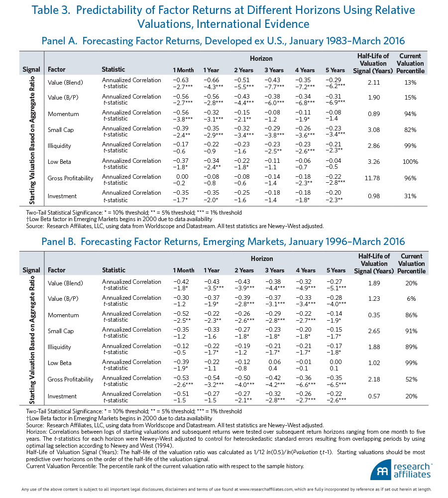
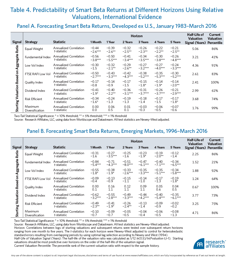
We now take our analysis out of sample, testing whether the relative valuations of factors and smart beta strategies are strongly correlated with factor returns globally, as they are in the United States. We are able to create factor/smart beta strategy returns and relative valuation measures back to 1983 for the developed world ex U.S. and to 1996 for emerging markets. For brevity we base these tests on the aggregate valuation measure only. We summarize our key findings, in Tables 3 and 4.14 All supporting data, as well as relative valuations using P/B, are available upon request. Across the eight factors and eight smart beta strategies, in both developed ex U.S. and emerging markets, and across most horizons, the relative valuations and future returns have overwhelmingly negative relationships.
In Table 3, of the 96 tests for factors, only 2 have the “wrong” sign, with higher valuation pointing to (negligibly) higher subsequent returns; both instances of the “wrong” sign are in the emerging markets, for which we have shorter history, and are for the low beta factor, for which the current valuations, in the 99th percentile, are quite extreme relative to history.
In Table 4, of the 96 tests for smart beta strategies, only 8 have the “wrong” sign: maximum diversification, over short horizons, in the developed ex U.S. region, and quality in the emerging markets. Incidentally, the current valuations for maximum diversification and the quality index are in the 99th and 100th percentiles, respectively; it is possible the high ending valuations over this sample lead to the lack of a negative relationship. Perhaps mean reversion for these strategies still lies in their future, at which point the typical negative relationship will become evident.
Weaker statistical significance is to be expected with a shorter history. For the 20-year span for emerging markets and the 33-year span for developed ex U.S. markets, information coefficients of 0.3 and 0.25, respectively, are typically sufficient for statistical significance at a two-tail 5% significance level. Two-thirds of the 192 results are statistically significant, and as with the U.S. results, over 40% are significant at the 1% level, despite a far shorter non-U.S. history. These results evidence a strong out-of-sample validation that relative valuations are indicative of future factor and smart beta strategy returns. Correlations for both factors and smart beta strategies are largely in line with those observed in the U.S. market. Interestingly, for value (using both definitions), momentum, and size, the relationship is quite strong despite the shorter time samples. When we compare U.S. and international results, the correlations are largely similar between strategies. The notable exceptions are slightly lower correlations in the cases of quality, maximum diversification, and risk efficient strategies.
In developed ex U.S. markets, profitability and low beta are weaker in statistical significance than in the United States. Quality, maximum diversification, and risk efficient strategies, which all have weaker correlations, also (not unsurprisingly) have weaker statistical significance. Is this because these factors and smart beta strategies are trading well into their highest valuation deciles ever (e.g., 96% for profitability and 100% for low beta, and in the top three deciles for the smart beta strategies) with no opportunity yet to mean revert? Perhaps.
The half-lives of valuations for factors are generally consistent with those observed in the United States with some interesting exceptions. Gross profitability, for example, has an extremely long half-life in the developed ex U.S. markets (11.78) compared to the U.S. market (3.09). The half-life of valuation signal in emerging markets tends to be shorter than in developed markets. The relationship is consistent for the smart beta strategies, whose half-lives are also generally shorter in the emerging markets.
Valuations Today: A Global Perspective
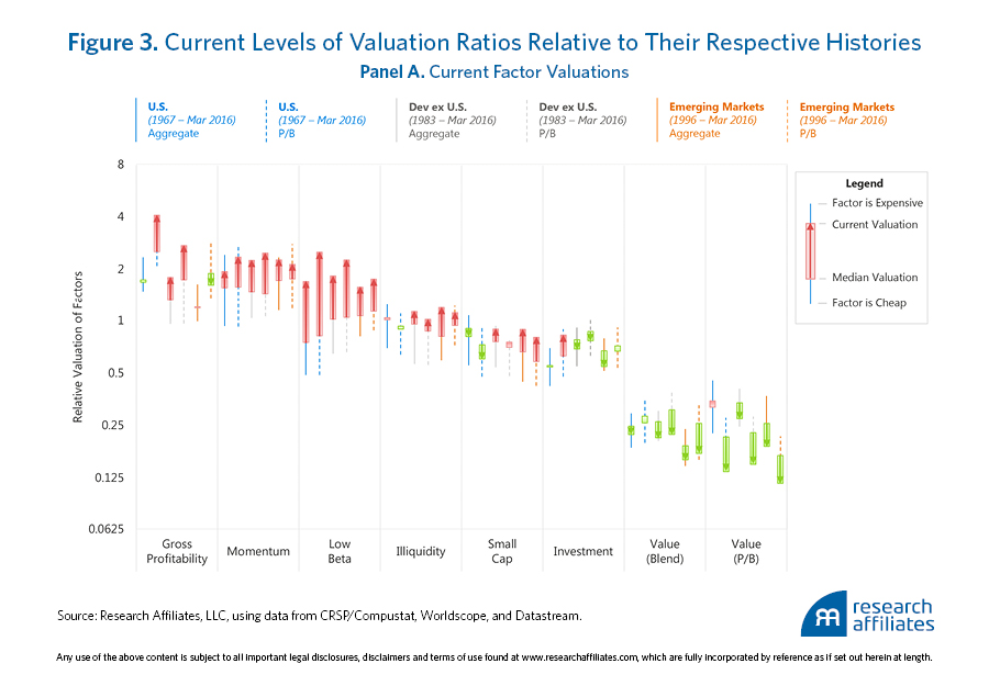
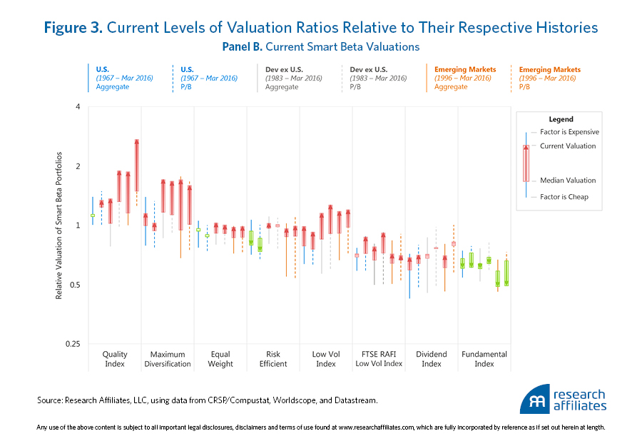
Now, let’s put our findings into context on a global scale. We compare, from highest average relative valuation to lowest, the current valuations for the eight factors and eight smart beta strategies in the U.S., developed ex U.S., and emerging markets, as shown in Figure 3. Value (using both forms, B/P and blended) falls in the bottom quintile of its historical valuation in both international and emerging markets; of 12 comparisons (U.S., international, and emerging markets, constructed using both B/P and the blended valuation, and with relative valuation measured versus both P/B and the aggregate measure), 11 suggest value is trading cheap, with 5 in the bottom decile of the historical valuation range. The investment factor (which correlates with value) is cheaper than its historical norm, though not by a wide margin. Small cap is a little cheap in the United States, but not elsewhere. Momentum, illiquidity, and low beta are all in the top quintile of their respective historical valuations in both international and emerging markets. In the international markets, gross profitability also falls into this category, but not so in the emerging markets. A casual examination of Figure 3 suggests that value is trading cheap in most domains and using most measures, while many of the factors attracting a flood of investment capital are trading rich. Dangerous? We think so, especially versus expectations based on the past 15 years.
Current valuation ratio percentiles of international smart beta strategies mirror U.S. smart beta strategies with two exceptions. The equal-weight strategy, priced just below its median historical valuation in the United States, is in the top quintile of its historical valuation in developed ex U.S. and emerging markets. This is consistent with small-cap stocks being relatively expensive internationally and cheap domestically. The other exception is the quality index, which, while sensibly priced in the U.S. market, is at all time high valuations in developed ex U.S. and emerging markets.
Conclusion
We have shown that the relative valuations of factors and smart beta strategies are strongly correlated with their respective future returns, not only in U.S. markets, but in markets around the world, for time horizons looking out to five years. We would offer a word of caution to those who wish to use these findings to aggressively time strategies: timing strategies leads to greater concentration of risk, so lacks diversification. A noisy signal and weak ability to diversify is a recipe for disappointment.
Having cautioned investors who may seek to aggressively time strategies in the direction of cheapness, we should note that chasing strategies with top quintile current valuation levels is even more dangerous. Many investors—including some very large, sophisticated investors—are already “timing” factors and strategies in the opposite direction, piling into the hottest new investment strategies, perhaps in an attempt to diversify risk away from their existing value strategies at a time when value is trading at historical valuation lows and some of the diversifying strategies are at historical highs. Why would investors do this? Because they don’t notice that brilliant past returns are a consequence of sky-high current valuations and may easily mistake those returns for structural alpha. Investors who wish to diversify away from past disappointment are, of course, welcome to do so—in reality, however, they are engaged in performance chasing and the desired diversification benefits may be illusory!
Investors who dismiss starting valuations, those who don’t look before they leap, remind us of the maxim “If you have to ask how much it is, you probably can’t afford it.” It’s a snobby comment that reeks of having so much money one can throw it around with abandon. People who ignore starting valuations in financial assets may unwittingly have that same imperious recklessness. Unlike the Vanderbilts and Carnegies of old, we’re confident most investors today don’t have money coming out of their ears. Pensions are underfunded (even with implausible return assumptions), 401(k) savers have inadequate balances, and “safe” assets like cash have become a stealth tax on wealth.
Today, many popular factors and smart beta strategies are quite expensive relative to their historic valuations. Charlie Munger once described Warren Buffet and his approach to investing this way: “It is remarkable how much long-term advantage people like us have gotten by trying to be consistently not stupid, instead of trying to be very intelligent. There must be some wisdom in the folk saying ‘It’s the strong swimmers who drown.’”
Some of the strategies currently commanding abnormal valuations may have become expensive because of the natural desire to outsmart the competition and to find the next big, shiny investment strategy. Some may have attracted this attention because they have become expensive for other reasons, a consequence of selection bias. Our research demonstrates that price matters, albeit with considerable noise and uncertainty. Before leaping into the next great strategy, do we really want to follow the counsel of many who argue that we should turn a blind eye to current valuation levels?
The next article in this series may perhaps be the most controversial: we will discuss the future returns that current valuation levels of factors and smart beta strategies around the world might be indicating. And, we show that a cautious dose of factor and smart beta strategy timing can, indeed, add some value. We hope we’ve piqued your interest!
Please read our disclosures concurrent with this publication: https://www.researchaffiliates.com/legal/disclosures#investment-adviser-disclosure-and-disclaimers.
Endnotes
- It bears mention that the previous article in this series stirred a certain amount of controversy. While we are amused at the hyperventilating in some of the reaction, we are deeply grateful for the feedback. To us, these critics serve as surrogate journal referees. Thank you.
- There is no generally accepted definition of “smart beta.” Our proposal, which we discuss in detail in “What ‘Smart Beta’ Means to Us” (Arnott and Kose 2014), combines one core criterion (it must overtly sever the link between the price of a stock and its weight in the portfolio) and several weaker requirements (the strategy must have most of the other advantages of conventional indexing, such as low turnover, broad market representation, liquidity, capacity, transparency, ease of testing, low fees, and so forth).
- It bears mention that Sanjoy Basu’s seminal paper on the value effect appeared in 1977 after an extraordinary five-year run in which the value effect both delivered exceptional returns, following the collapse of the Nifty Fifty, and saw an exceptional rise in relative valuation to levels, at least on the basis of P/B, never seen since. Only about 10% of the half-century of benefits from the value effect was earned in the nearly 40 years after Basu’s paper was published; 90% predates publication. Was Basu engaged in inadvertent data mining, finding the value effect after, and because of, a surge in both relative valuation and relative performance? Probably. It assuredly wasn’t deliberate and the “wedge” between relative valuation and relative performance would suggest that the value effect has merit. Still, his was the first of many factors discovered near historical peaks of relative valuation, delivering comparatively little reward since they were first published. Caveat emptor.
- Look-ahead modeling bias is an important issue that can render variables, even those having good in-sample correlation with subsequent returns, to be extremely weak as an out-of-sample conditioning variable. Goyal and Welch (2003) demonstrate this point using market-wide dividend yield to forecast subsequent market performance. In the third article of our series, we’ll deal with this nuance. It makes surprisingly little difference when results are as robust across markets and time spans as these. We will explore the merits of ex ante valuation-based forecasts in predicting factor returns. And we will show that factor or strategy timing is useful, if we pursue it with due caution.
- Cheapness can be due to a higher perceived risk associated with value companies or may be associated with mispricing. Generations of academics have argued about the cause without much success in resolving the debate. Regardless of which camp is right, the value effect is still present.
- In each of these cases our replication follows the published methodology. In the live implementation of the products based on these methodologies, investment managers may introduce significant modifications. These modifications can make live product investment characteristics quite different from published methodologies and, consequently, from our replication. We encourage potential investors interested in the products to learn the performance and the portfolio characteristics of the actual products coming from their corresponding product providers.
- Charts plotting relative performance versus relative valuation for each of the six factors can be found in the first article “How Can ‘Smart Beta’ Go Horribly Wrong?”. Value, momentum, size, and illiquidity all show a notable wedge. Each likely has a powerful structural alpha, which can be masked by falling valuation levels or by anomalous short-term results. The same cannot be said for low beta or profitability.
- A detail-oriented reader will notice that valuations may mean-revert due to either price changes or to portfolio turnover. When we explain the intuition behind half-life of valuation mean reversion in this article, we assume the second effect is significantly stronger.
- A 20% correlation with monthly returns is, for example, vastly more useful than a 20% correlation with five-year returns. We divide our correlations by the square root of the time horizon, adjusting all correlations to an annualized equivalent to create an apples-to-apples comparison. An adjustment for the serial correlation of returns accomplishes much the same thing. The adjustment is an approximation using a simplified assumption that returns are not serially correlated between subperiods. This approximation breaks down for large levels of correlation; for example, if the monthly correlation is above 0.29, the annualized correlation computed using our method will be above 1.0, which is, obviously, impossible. Nevertheless, for the low levels of correlation we observe here, it is a useful approximation that allows us to make effective comparisons between disparate correlations measured on different horizons.
- Others, such as Asness et al. (2000) and Cohen, Polk, and Vuolteenaho (2003), demonstrate this approach works for the value factor. Li and Lawton (2014) and Garcia-Feijóo et al. (2015) demonstrate that valuations are extremely important for low beta/low volatility strategies. Asness, Frazzini, and Pedersen (2013) show that valuations predict the future quality-minus-junk factor return they study in the article. Our new findings show the same principle works for almost any strategy. Recently, Dai (2016) shows that valuations can be predictive of market, value, size and profitability factor returns. Relative valuation is not the only variable demonstrated to be correlated with subsequent factor performance. Daniel and Moskowitz (2013) and Barroso and Santa-Clara (2014) show that extreme volatility tends to be predictive of subsequent momentum crashes and Granger et al. (2014) show how optionality imbedded in a rebalancing strategy is a timing mechanism that can help generate a higher return and a higher Sharpe ratio, albeit at a cost of altering higher moments.
- We observe that P/B-based valuation does a better job of forecasting the return of the value blend factor, whereas the aggregate valuation measure does a better job of forecasting the return of the value strategy constructed based on B/P. An explanation may be that the P/B ratio has a better ability to forecast junk rallies, or those periods when recently unprofitable and highly distressed companies are valued by the market at unjustifiably low levels and sharply revert even on the slightest of positive news. The value factor formed on B/P is likely to load on low profitability/junk companies, whereas the aggregate valuation metric may be better at identifying quality and thus may do a better job of predicting the subsequent return. The value strategy constructed using a composite measure, however, has an imbedded tilt toward companies with higher profitability; that is, when the book-to-market spread is the largest, all value companies probably do well, but more profitable value companies likely do better than average. An alternative explanation may be that when the same variable is used to construct and measure the cheapness of the strategy, the valuation signal becomes noisier.
- An example of this phenomenon, from our 1967 starting point, is when the value effect had cumulative statistical significance that was lousy at the peak of the tech bubble and the trough of the global financial crisis, but was impressive from 2004 to 2007. Did the value effect lose, then gain, then lose statistical significance? Or was a statistical estimate of its efficacy affected by our choice of end date, understated in 2000 and 2009, and overstated in 2004–2007? Was each estimate of the power of the value effect subject to its own estimation error, overlooked by much of the quant community at their peril? The lofty significance in 2004–2007 helped drive the soaring popularity of leveraged quant strategies, which “crashed” in August 2007.
- Critics have suggested this comparison does not make sense for factors with a constantly changing composition, such as the momentum and low beta factors. In our first article, we note the turnover of these strategies, pointing out the weak relationship. Let’s not throw the baby out with the bath water. For such strategies, we show the starting valuation is a surprisingly powerful indicator of future returns, even though the portfolios change rapidly over time. In our upcoming third article, we will expand on the half-life of factors and smart beta strategies as a gauge of how quickly current relative valuations can become irrelevant.
- Generally, we observe stronger correlations with future returns when we use aggregate relative valuation measures compared to using P/B alone.
References
Amenc, Noël, Felix Goltz, Lionel Martellini, and Patrice Retkowsky. 2010. “Efficient Indexation: An Alternative to Cap-Weighted Indices.” EDHEC-Risk Institute (January).
Amihud, Yakov. 2002. “Illiquidity and Stock Returns: Cross-Section and Time-Series Effects.” Journal of Financial Markets, vol. 5, no. 1 (January):31–56.
Arnott, Robert D., and Peter L. Bernstein. 2002. “What Risk Premium Is ‘Normal’?” Financial Analysts Journal, vol. 58, no. 2 (March/April):64–85.
Arnott, Robert D., Jason Hsu, and Philip Moore. 2005. “Fundamental Indexation.” Financial Analysts Journal, vol. 61, no. 2 (March/April):83–99.
Arnott, Robert D., and Engin Kose. 2014. “What ‘Smart Beta’ Means to Us.” Research Affiliates Fundamentals (August).
Asness, Clifford S., Andrea Frazzini, and Lasse Heje Pedersen. 2014. “Quality Minus Junk.” (June 19). Available on SSRN.
Asness, Clifford S., Jacques A. Friedman, Robert J. Krail, and John M. Liew. 2000. “Style Timing: Value versus Growth.” Journal of Portfolio Management, vol. 26, no. 3 (Spring):50–60.
Barroso, Pedro, and Pedro Santa-Clara. 2014. “Momentum Has Its Moments.” Journal of Financial Economics, vol. 116, no. 1 (November):111–120.
Basu, Sanjoy. 1977. “Investment Performance of Common Stocks in Relation to Their Price-Earnings Ratios: A Test of the Efficient Market Hypothesis.” Journal of Finance, vol. 32, no. 3 (June):663–682.
Choueifaty, Yves, and Yves Coignard. 2008. “Toward Maximum Diversification.” Journal of Portfolio Management, vol. 35, no. 1 (Fall):40–51.
Cohen, Randolph B., Christopher Polk, and Tuomo Vuolteenaho. 2003. “The Value Spread.” Journal of Finance, vol. 58, no. 2 (April):609–642.
Dai, Wei. 2016. “Premium Timing with Valuation Ratios.” Dimensional Fund Advisors white paper (March).
Daniel, Kent D., and Tobias J. Moskowitz. 2013. “Momentum Crashes.” Swiss Finance Institute Research Paper No. 13-61; Columbia Business School Research Paper No. 14-6; Fama–Miller Working Paper (September 30).
Fama, Eugene, and Kenneth French. 1993. “Common Risk Factors in the Returns on Stocks and Bonds.” Journal of Financial Economics, vol. 33, no. 1 (February):3–56.
———. 2002. “The Equity Premium.” Journal of Finance, vol. 57, no. 2. (April):637–659.
———. 2012. “Size, Value, and Momentum in International Stock Returns.” Journal of Financial Economics, vol. 105, no. 3 (September): 457-472.
———. 2015. “A Five-Factor Asset Pricing Model.” Journal of Financial Economics, vol. 116, no. 1 (April):1–22.
Frazzini, Andrea, and Lasse H. Pedersen. 2014. “Betting Against Beta.” Journal of Financial Economics, vol. 111, no. 1 (January):1–25.
Garcia-Feijóo, Luis, Lawrence Kochard, Rodney N. Sullivan, and Peng Wang. 2015. “Low-Volatility Cycles: The Influence of Valuation and Momentum on Low-Volatility Portfolios.” Financial Analysts Journal, vol. 71, no. 3 (May/June):47–60.
Goyal, Amit, and Ivo Welch. 2003. “Predicting the Equity Premium with Dividend Ratios.” Management Science, vol. 49, no. 5 (May):639–654.
Granger, Nicolas M., Douglas Greenig, Campbell R. Harvey, Sandy Rattray, and David Zou. 2014. “Rebalancing Risk.” (October 3). Available on SSRN.
Hsu, Jason, Brett W. Myers, and Ryan Whitby. 2016. “Timing Poorly: A Guide to Generating Poor Returns While Investing in Successful Strategies.” Journal of Portfolio Management, vol. 42, no. 2 (Winter):90–98.
Li, Feifei, and Philip Lawton. 2014. “True Grit: The Durable Low Volatility Effect.” Research Affiliates Fundamentals (September).
Newey, Whitney K., and Kenneth D. West. 1994. “Automatic Lag Selection in Covariance Matrix Estimation,” Review of Economic Studies, vol. 61 (April), 631–653.
Simulation Methodology Used in “To Win with ‘Smart Beta’ Ask If the Price Is Right”
For Factors
For factor simulations in the United States we use the universe of U.S. stocks from the CRSP/Compustat Merged Database. We define the U.S. large-cap equity universe as stocks whose market capitalizations are greater than the median market-cap on the NYSE. For international factors (developed ex U.S. and emerging markets) we use the universe of stocks from the Worldscope/Datastream Merged Database. We define the international large-cap equity universe as stocks whose market-caps put them in the top 90% by cumulative market-cap within their region, where regions are defined as North America, Japan, Asia Pacific, Europe, and Emerging Markets.
The large-cap universe is then subdivided by various factor signals to construct high-characteristic and low-characteristic portfolios, following Fama and French (1993) for the U.S. and Fama and French (2012) for international markets (Note that slight variations in data cleaning and lagging, as well as different rebalance dates, could lead to slight differences between our factors and those of Fama and French). As an example, in order to simulate the value factor in the United States, we construct the value stock portfolio from stocks above the 70th percentile on the NYSE by book-to-market ratio, and we construct the growth stock portfolio from stocks below the 30th percentile by the same measure. Internationally, we construct the value stock portfolio from stocks above the 70th percentile in their region (North America, Japan, Asia Pacific, Europe, and Emerging Markets) by book-to-market, and the growth stock portfolio from stocks below the 30th percentile in their region.
The stocks are then market-cap weighted within each of the two portfolios, which are used to form a long–short factor portfolio. Portfolios are rebalanced annually each January with the exception of momentum, which is rebalanced monthly. U.S. data extend from January 1967 to March 2016, developed ex U.S. from January 1983 to March 2016, and emerging markets from January 1996 to March 2016, and has been filtered to exclude ETFs and uninvestable securities such as state-owned enterprises and stocks with little to no liquidity. The signals used to sort the various factor portfolios follow:

For Smart Beta Strategies
We use the universe of stocks of the top 1,000 U.S., developed ex U.S., and emerging markets companies by market capitalization for all smart betas with the exception of Fundamental Index™, for which we use the top 1,000 companies by fundamental size. The portfolios are defined as follows:

